DENLDuffing

Duffing Non Linear Differential Equation

Differential Equation Non Linear Duffing

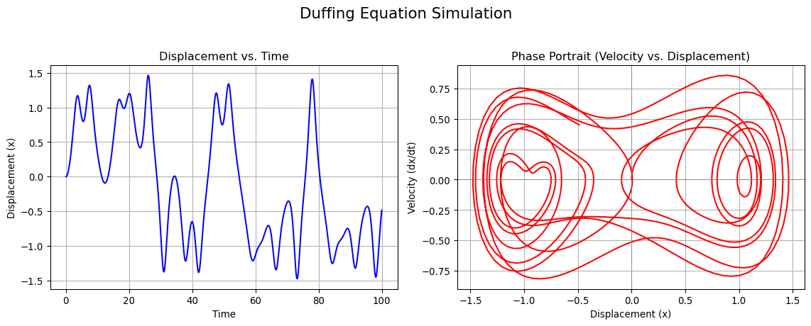
import numpy as np
from scipy.integrate import odeint
import matplotlib.pyplot as plt

# --- 1. Define the Duffing Equation as a system of first-order ODEs ---
# The Duffing equation is a second-order non-linear differential equation:
#  x'' + delta*x' + beta*x + alpha*x^3 = gamma*cos(omega*t)
# We convert it to a system of two first-order ODEs for numerical solution:
# Let y[0] = x (displacement)
# Let y[1] = x' (velocity)
# Then, y[0]' = y[1]
# And, y[1]' = gamma*cos(omega*t) - delta*y[1] - beta*y[0] - alpha*y[0]**3

def duffing_model(y, t, delta, alpha, beta, gamma, omega):
    """
    Returns the derivatives of the state variables for the Duffing equation.

    Args:
        y (list): A list or array containing the state variables [x, x'].
        t (float): The current time.
        delta (float): Damping coefficient.
        alpha (float): Coefficient for the non-linear term.
        beta (float): Coefficient for the linear restoring force.
        gamma (float): Amplitude of the periodic forcing term.
        omega (float): Frequency of the periodic forcing term.

    Returns:
        list: The derivatives of the state variables [x', x''].
    """
    y0_prime = y[1]
    y1_prime = gamma * np.cos(omega * t) - delta * y[1] - beta * y[0] - alpha * y[0]**3
    return [y0_prime, y1_prime]

# --- 2. Set up the parameters and initial conditions ---
# Parameters for the Duffing oscillator
delta = 0.2  # Damping
alpha = 1.0  # Non-linear spring coefficient
beta = -1.0  # Linear spring coefficient (negative for a bistable potential)
gamma = 0.3  # Forcing amplitude
omega = 1.0  # Forcing frequency

# Initial conditions [x(0), x'(0)]
y0 = [0.0, 0.0]

# Time points to solve for
t = np.linspace(0, 100, 1000)

# Pack parameters into a tuple
params = (delta, alpha, beta, gamma, omega)

# --- 3. Solve the ODE using odeint ---
# The odeint function returns an array where each row is a solution for a time point.
solution = odeint(duffing_model, y0, t, args=params)

# --- 4. Plot the results ---
# Separate the solution into displacement (x) and velocity (x')
x_solution = solution[:, 0]
x_prime_solution = solution[:, 1]

# Create a figure with two subplots side-by-side
fig, (ax1, ax2) = plt.subplots(1, 2, figsize=(12, 5))
fig.suptitle('Duffing Equation Simulation', fontsize=16)

# Plot Displacement vs. Time
ax1.plot(t, x_solution, 'b-')
ax1.set_title('Displacement vs. Time')
ax1.set_xlabel('Time')
ax1.set_ylabel('Displacement (x)')
ax1.grid(True)

# Plot the Phase Portrait (Velocity vs. Displacement)
ax2.plot(x_solution, x_prime_solution, 'r-')
ax2.set_title('Phase Portrait (Velocity vs. Displacement)')
ax2.set_xlabel('Displacement (x)')
ax2.set_ylabel('Velocity (dx/dt)')
ax2.grid(True)
ax2.axhline(0, color='gray', linewidth=0.5)
ax2.axvline(0, color='gray', linewidth=0.5)

# Adjust layout and display the plots
plt.tight_layout(rect=[0, 0.03, 1, 0.95])
plt.show()